Classification of Power Plants: CNN vs. General Regression Model
This article is a project from Machine Learning course: CS 229 at Stanford University. This project was aimed at exploring different machine learning frameworks and analyzing pros and cons of different models.
Background
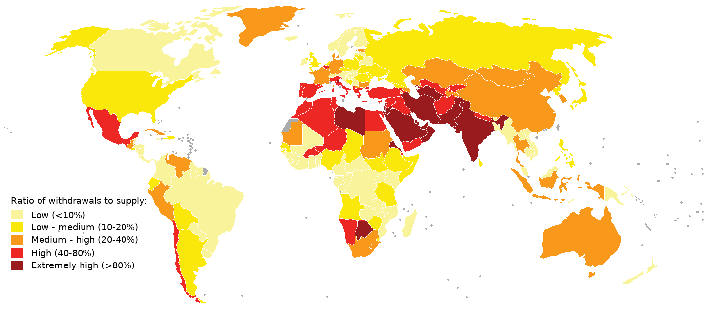
The energy sector is the second-largest consumer of water globally. In an era of growing concern around water risk, stakeholders are interested in quantifying water use by thermal power plants. In 2016 the World Resources Institute (WRI) created a new methodology that combines reported energy use data and power plant characteristics to generate estimates for water consumption by plant, and applied the methodology to over 85% (by installed capacity) of the Indian thermal energy sector. The methodology relied on individual inspection of power plants via satellite-based images. These inspections sought to classify power plants by cooling type, as different cooling types have significantly different visual features from satellite images, and the cooling types were used in turn to help characterize water consumption.
Motivation
Visual inspection offers a reliable result of cooling type, but it is time-consuming. In order to generalize WRI’s methodology, the previously classified Indian plant data set can be used to build a machine learning model which can automatically classify plant cooling type and can be used for future uses if the results are reliable. In this project, we use different machine learning models to build a classifier that can predict the cooling types well.
Dataset & Features
We worked with a dataset of over 350 Indian power plants, which included multiple numerical and categorical labels such as: GPS location of the plant, presence or absence of each of the four cooling types, fuel type, installed capacity, plant capacity type, Indian State, Power Plant Parent Company, etc. (provided in a CSV file)These data were compiled both from visual inspection of satellite data and from existing commercial and public databases, made available by WRI. We manually confirmed the GPS locations for every power plant in our database, updating when appropriate and discarding if the location did not correspond to an actual power plant.
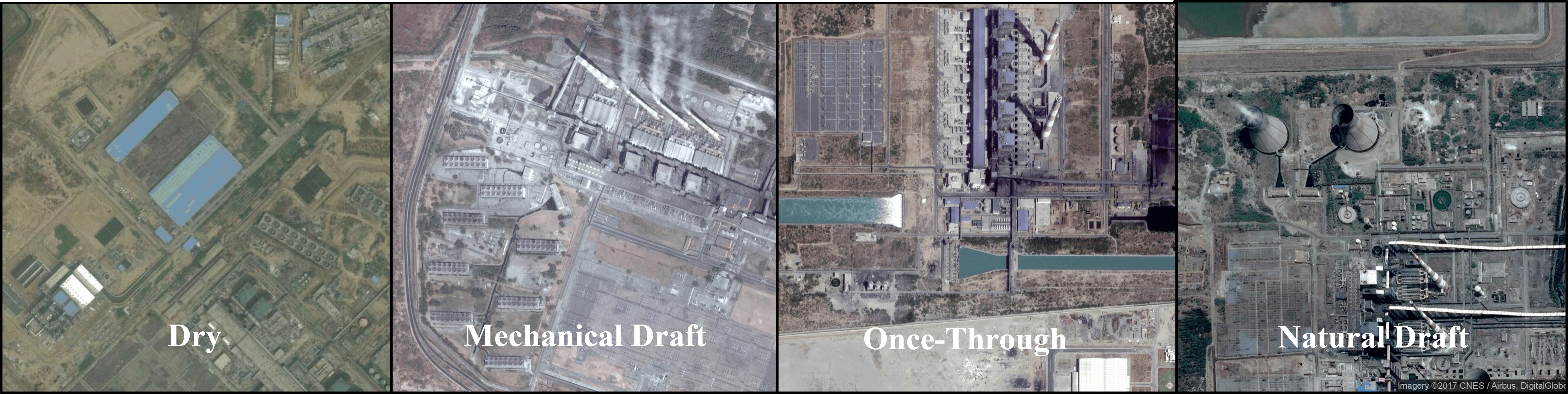
From visual inspection, the following are the key image features that characterize type of plants:
- Dry: rectangular tile on black
- Mechanical Draft: aligned circular plates
- Once-Through: existence of artificial dam (river near power plant)
- Natural Draft: cooling tower towering in a chimney shape
Problem Forumlation
We used two separate models to test the prediction model: Binomial Logistic Regression and ConvNet based on transfer learning with the MobileNet model. For both our logistic regression and neural net, we chose to use four binomial models to predict our four cooling types, rather than using a single multinomial model. We chose four binomial models because some power plants use two different cooling types rather than a single cooling type, which makes it a multi-label classification problem, reducing the model accuracy to classify each plant or image of a plant as containing strictly one cooling type.
Model 1: Binomial logistic regression
The logistic regression models use numerical and categorical features other than GPS locations, such as:- fuel type
- installed thermal capacity
- Plant Capacity Factor (PCF)
- etc.
To build a training model that best predicts the plant's cooling type, we used one-vs-one method for binary classification and used k-fold cross validation to randomly sample from the dataset to select the best set of data that has less bias than others. In our binomial logistic regression model, we used the following configuration:
| Training Set | n = 230 |
|---|---|
| Test Set | n = 80 |
| k-fold Cross Validation | k = 10 |
| Number of Iterations | Iteration = 30 |
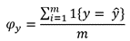
For each of our four binomial outputs (cooling type), we performed 30 iterations of 10-fold cross validation on various models. Multiple cross validations were conducted to obtain the best dataset that captures the characteristic of the model that best predicts the cooling type. We used a simple function which returned 1 for a correct prediction and 0 for an incorrect prediction, averaged over all predictions (Equation 2). After selecting the four models with the best 10-fold cross validation accuracy, we predicted on the test set and reported the accuracy.
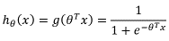
Our logistic regression model used python sklearn.multiclass package OneVsOneClassifier. which takes in labeled dataset so that sigmoid function is applied to a linear combination of the features to generate a number between 0 and 1. The sigmoid output is treated as a probability as shown in the following equation. When it is greater than 0.5, we predict the presence of the modeled cooling type, and when it is less than 0.5 we predict its absence.
To measure accuracy, we used a simple function which returned 1 for a correct prediction and 0 for an incorrect prediction, averaged over all predictions as shown in equation below. After selecting the four models with the best 10-fold cross validation accuracy, we predicted on the test set to test the accuracy.
Classification Results
Results from our logistic regression model are presented in Table 1 below. Results for dry cooling in particular, as well as natural draft and once-through are promising. Almost 20% of our data have missing GPS coordinates, so our ability to predict cooling type based on other available features is an important contribution to data imputation for this class of problem. Mechanical draft prediction underperforms other categories--we believe the other parameters simply do not contain sufficient information to predict mechanical draft cooling with high accuracy.
| Mechanical Draft | Natural Draft | Dry | Once-Through | |
|---|---|---|---|---|
| Cross Validation Accuracy | 65% | 82% | 86% | 94% |
| Test Accuracy | 71.25% | 78.75% | 88.75% | 82.50% |
Model 2: Image classification using MobileNet architecture
Our second model uses the general architecture of MobileNets, a streamlined CNN architecture that uses depth-wise separable convolutions to build light-weight deep neural networks. We selected MobileNet for its relative speed and simplicity, which allowed us both to rapidly prototype and iterate, and was appropriate given our small volume of data. Also, as many ConvNets are parameter-rich and pront to overfitting, we selected a simpler ConvNet with a smaller parameter space.
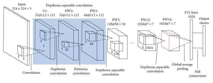
We managed the entire retraining process via Tensorflow’s recommended retrain.py script, which also features easy methods to control gradient descent batch size, train/dev/test size, and certain distortions. Finally, in our implementation of the MobileNet model, the weights for every layer were maintained except for the last fully-connected layer to retrain this layer on our images.
Data Augmentation by image distortions
Image distortions act in a manner similar to regularization, forcing the ConvNet to generalize rather than simply “memorizing” the training set. This technique is used extensively in image classification in order to overcome small number of datasets and overfitting. We can take advantage of this technique to overcome overfitting problem due to our small number of datasets (n = 350). We do this by varying the following:
- image offsets
- size scaling
- brightness
- orientation (left/right switching)
The application of distortions increased our computational time by several orders of magnitude, and had little effect at low levels, but with 80% random offsets, random scaling, and random brightness in addition to random left/right switching we were able to bring our dev set accuracy up to almost 70%.
Classification Results
Results from our ConvNet are presented in Table 2. Training and development set numbers reflect the values to which the training and development set accuracies converged. Results for natural draft, dry, and once-through cooling types surpassed results from our logistic regression model (after correct pre-processing was applied).
| Mechanical Draft | Natural Draft | Dry | Once-Through | |
|---|---|---|---|---|
| Training Accuracy | 100% | 100% | 100% | 100% |
| Test Accuracy (N = 84) | 68.8% | 98.9% | 62.5% | 61.4% |
We found that the results for mechanical draft cooling are disappointing, as humans can identify mechanical draft cooling structures with high (>95%) accuracy. As it can be seen from Figure 2, our mechanical draft model suffers badly from overfitting.
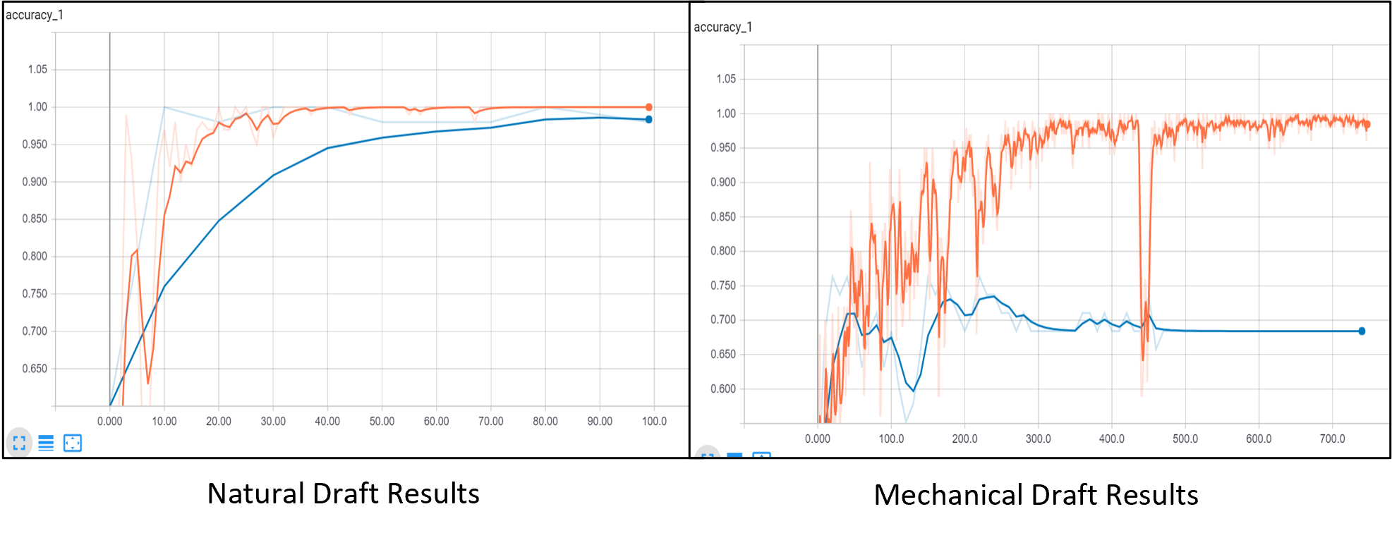
Our original dev set accuracies were as low as 55% while training set accuracies converged to 100%. To solve this overfitting problem we tried a number of steps, including simpler model selection and random image distortions applied to training samples before each batch iteration.
Potential factors in misclassification
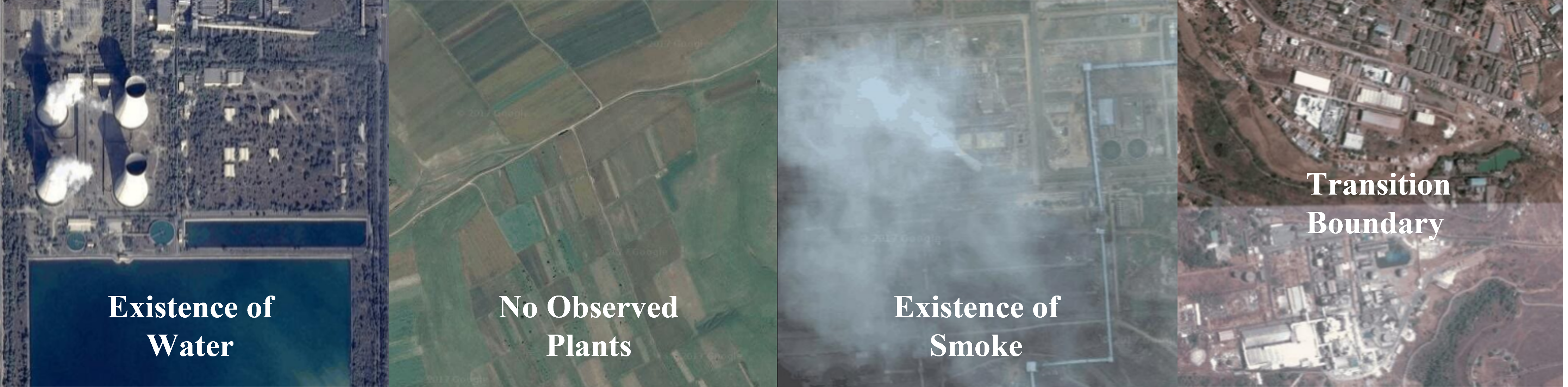
It could be seen that:
- Existence of Water for Natural Drafts: Natural Draft that has rivers and oceans nearby could be misclassified as once-through
- No Observed Plants: If the power plant is missing or far from the given coordinates
- Existence of Smoke: Circular plate characteristic of Mechanical Draft is not visible
- Transition Boundary: When satellite images are taken at different times, different tones are created
Discussion on model performance
The ConvNet uses a satellite image of the power plant as input to predict plant cooling type, as each cooling type is associated with specific visual characteristics. Our ConvNet is more accurate, but requires the plant’s GPS location. Even our own data contains many instances where GPS data is missing or inaccurate--under these conditions, our logistic regression model generates a useful estimate for cooling type.
Unfortunately, we were unable to apply conventional regularization, as MobileNets is explicitly designed with minimal regularization (due to its already small parameter space) and our workflow did not allow a simple method to directly modify our weights’ update rules. Note the stochasticity of our accuracy in Figure 2--despite greatly reducing the learning rate, we were unable to find a smooth learning rate that did not require an infeasible number of iterations to convergence.
Conclusion / General comments
Our two models offer successful methods for classifying cooling types under a variety of conditions. When GPS coordinates are not available, our logistic regression model offers an acceptable “best guess” given there is no current human-driven methodology to estimate cooling types from other features. When GPS coordinates are available, our ConvNet offers classification on par with human classification for 3 of the 4 plant cooling types. Future opportunities include deeper changes to the MobileNets architecture in order to address the variance problem for mechanical draft prediction (e.g. the addition of L2 regularization).