MACHINE LEARNING APPROACH TO KINODYNAMIC MOTION PLANNING

Background

Autonomous robots, just like humans, can be defined as agents that can make their own decisions and then perform actions accordingly. A truly autonomous robot is one that can:

1. perceive its environment
2. make decisions, based on what it perceives, and/or has been programmed to recognize, and then actuate a movement or manipulation within that environment

With respect to robot mobility, for example, these decision-based actions include, but are not limited to, basic tasks like starting, stopping, and maneuvering around obstacles that are in their way. In order for robots to autonomously carry out these tasks, they would have to be robust against unexpected situations by quickly recognizing important changes in the environment, and act accordingly to properly respond to a situation. Understanding the dynamics of robots allows engineers to build a controller that can make intelligent controls such as collision avoidance and optimized path planning.

Optimization-based control theory

In control theory, there is a field called optimal control, a branch of mathematical optimization that deals with finding a control for a dynamical system over a period of time such that an objective function is optimized. Optimal control asks to compute a control function (either open loop or closed loop) that optimizes some performance metric regarding the control and the predicted state. For example, a driver of a car would like to reach a desired location while achieving several other goals: e.g., avoiding obstacles, not driving erratically, maintaining a comfortable level of acceleration for human passengers. Optimal control allows a control designer to specify the dynamic model and the desired outcomes, and the algorithm will compute an optimized control. This relieves some burden by letting the designer reason at the level of what the robot should do, rather than designing how it should do it. However, because the optimal control problem is a continuous problem, implementing the controller with a computer program wouldn't be feasible. Therefore, the solution is discretized into smaller intervals, making it an optimization-based control problem. An optimization-based control problem can be expressed in an objective form as follows:

where x is the state of the agent or robot and u is the control inputs, both in vector form. A and B are matrices which map the position and control input into the rate of change in the state of the agent.

Kino-dynamic Constraint

Can a robot, for example, a dubin vehicle, as shown in Figure 1, reach a desired end position by traveling in a straight line?

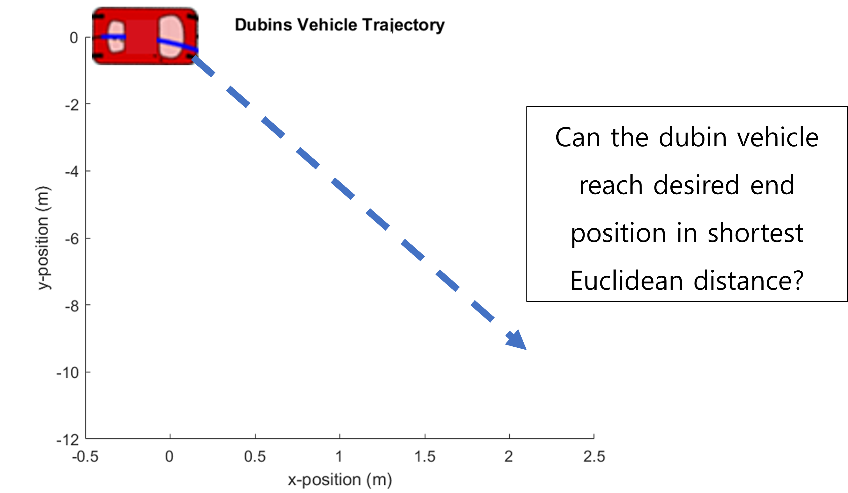
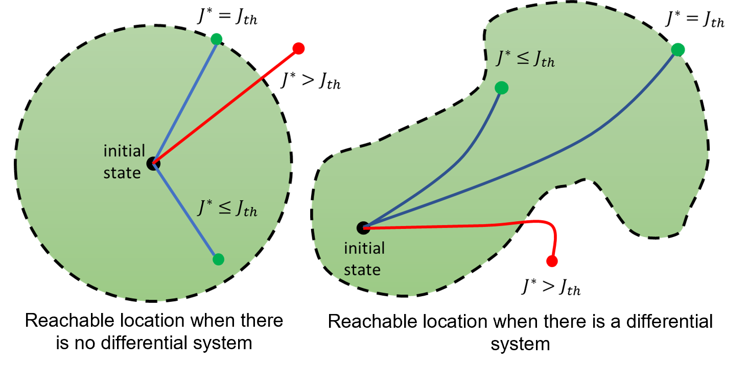
The answer is no. From experience, we have seen that even the strongest robots cannot instantaneously change velocities, and driving and flying robots cannot move sideways. This is because robots such as this dubin vehicle are kinematically and dynamically constrained in their motions. In automatic control theory research, there is a need to find an optimization-based open-loop control law that solves an optimization problem accounting kinodynamic (kinematic + dynamic) constraints. As shown in the image below, unlike the reachable sets where no differential system exists, there will be a different set of locations when there is a differential system.

Objective

Our goal is to implement the optimization-based control on the robot so that it can navigate its way towards its desired position while cost-effectively using minimum amount of fuel and traveling minimum amount of distance. How we do this is by solving the optimization problem above. However, computing the series of optimization problem would be computationally expensive and therefore would not be an appropriate control system for real-time planning. Therefore, a sampling-based method coupled with machine learning algorithms could significantly reduce the computational time required to calculate the online trajectory planning. Here we present the general framework to the problem.

In order to solve the above problem with convex optimization, this continuous problem is discretized using chebyshev pseudo-spectral method, making it a non-linear optimization problem. It is then transformed into a se

GOAL

Maneuver robots from one position to another position in real time, given that we fully know the environment.

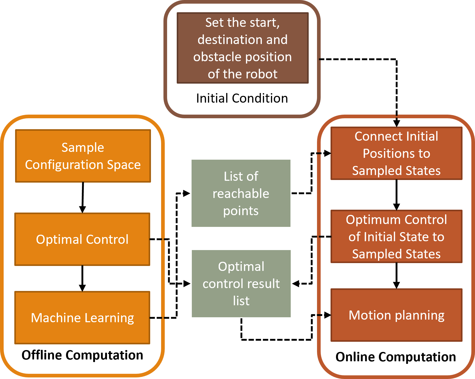
OFFLINE COMPUTATION

1. Sample the configuration space in the environment: we randomly pick n number of points in the configuration space, or the space of possible positions that a physical system may attain, possibly subject to external constraints.
2. Attain all possible 2-pair combination of the sampled states
3. Obtain trajectory path for each pair, solving an optimization-based control
4. Obtain how much time it takes to maneuver from one sampled location to the other location and save them into a dataset
5. Train the dataset using machine learning to obtain unknown reachable sets
6. Create a look-up table which is used for motion planning in online computation

ONLINE COMPUTATION

1. Set the initial and end position of the robot in the environment
2. Connect each of the start and end position to is closest sampled states respectively
3. Obtain trajectory path from start position to the closest state
4. Run a motion planning algorithm to find the best path, then navigate

It takes a lot of time to obtain a trajectory path for each pair by solving an optimization-based control, which means that when the initial conditions of the robot are given, it is impossible to grasp the path of the robot in a short time.

By Utilizing the "reachable distances" as data at a point, From these sampled points, we can see everything that can be reached from one point to another. The distance a robot can reach depends on how we set the distance threshold. Setting the threshold as high as above would allow the robot to move to more places online. In the long run, this could be more beneficial as it has more options of trajectories, but when a sudden blockage happens, it could cause trouble in the motion planning. On the other hand, if the distance threshold is set as low as below, it is suitable for short-term motion planning as only the shortest distances are selected that could be used for motion planning.

DATA PREPARATION

In order to obtain the trajectory, we would have to solve the optimization problem. For this problem, we will be using a dubin vehicle dynamics. The kinematics of the dubin vehicle is shown as follows:

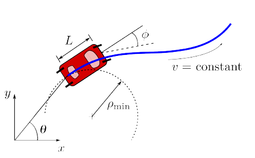
where the velocity is held constant (v = constant) and where angular velocity $\stackrel{·}{𝜃}$ is determined by the velocity and the angle (∅) of action taken by the robot. The only control input is the turnrate $\stackrel{·}{𝜃}$. Our objective function can be simplified as:

In order to solve this problem, we first discretize the space using chebyshev pseudo-spectral method, making it a non-linear optimization problem. It is then transformed into a series of convex optimization problems using Sequential Quadratic Programming (SQP). The scope of this article will not cover these in detail. All there is to know is that using some computationally expensive control inputs, we get a list of reachable points, stored as a data set, which will later be used to determine other unknown data points.

If we solve the optimization problem using the abovementioned algorithm (discretization and SQP), we will get a trajectory of the dubin vehicle position(x, y, t) and control inputs $\stackrel{·}{𝜃}$(t).

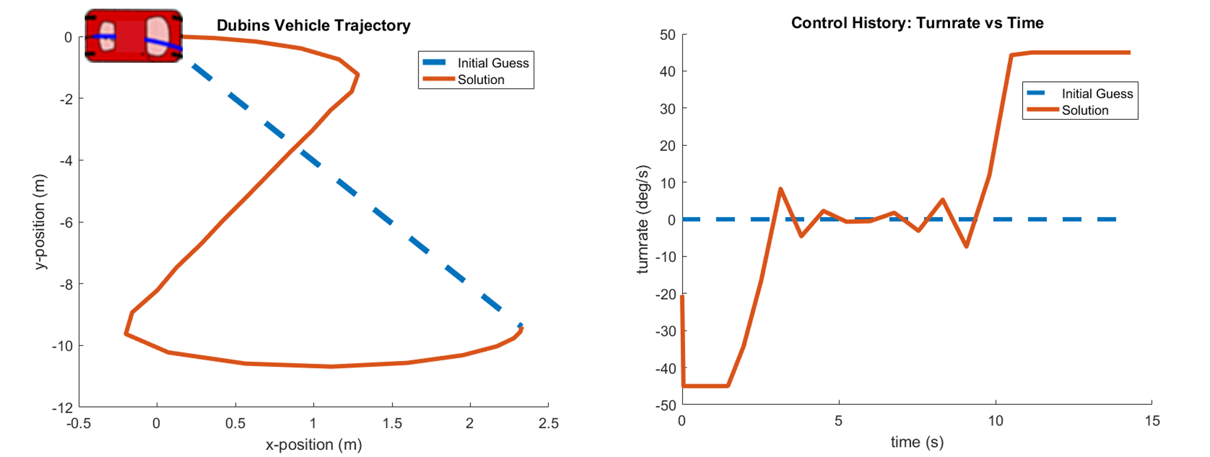
When the optimal control is performed to reach the final state (x, y, theta) = (2.3267, -9.3934, 90.927 deg) in the initial state (x, y, theta) = (0,0,0 deg) (Blue dotted line: initial guess, orange solid line: calculated distance). In order for such a robot to go to an optimized path, xit must go through a path with differential limitation.

REACHABILITY ANALYSIS USING WEIGHTED LINEAR REGRESSION

Instead of computing all possible states using optimization programming, we use the locally weighted linear regression to obtain the reachable sets. After sampling through sufficient pairs (n = 100), it was found that there was a linearly separable relationship between the reachable sets and the non-reachable sets given a user-defined threshold. The results are shown below:

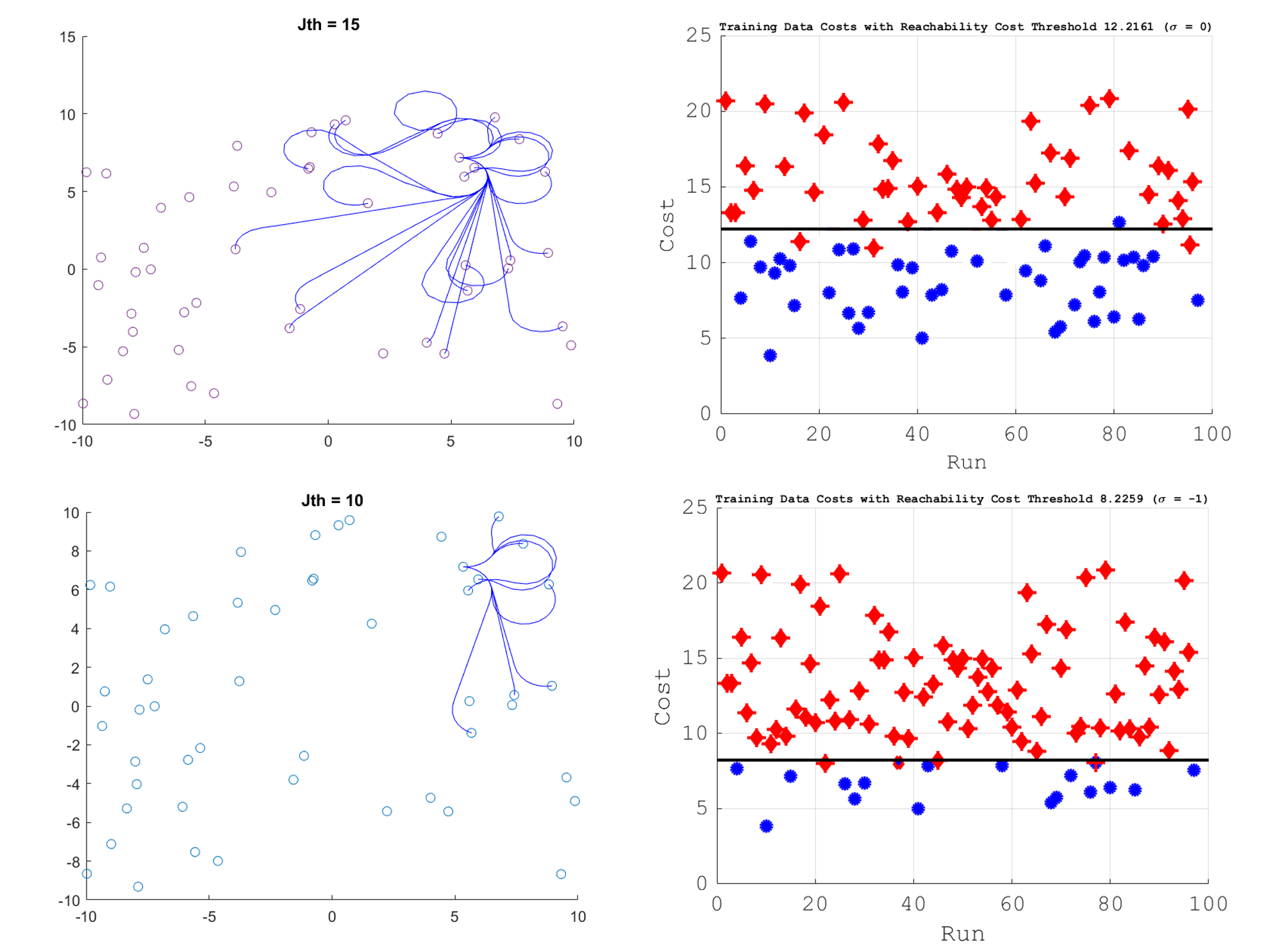
The red dots indicate non-reachable sets and the blue dots indicate reachable sets. As seen in the result, we can see that by lowering the cost threshold, the number of reachable sets decreases. There were some results that were not linearly separable, such that some values were classified as unreachable when it is in fact reachable.

APPLICATION: MULTI-AGENT PATH PLANNING

If we want two dubin vehicles to maneuver around the environment with the sampled states, we can add another reachability constraint such that each robot should choose a path that minimizes the likeliness of two paths colliding. After setting a starting point and ending point for each robot, we then obtain the closest reachable set for each and if they are the same, each robot takes a different set, They do this ahead of time because all states are observable (the robots don’t have to make real-time decisions because all states are already sampled). If no other states exist for one robot, the robot that has an alternative path can take the sampled state so that the robot with no other states can move to its only reachable set. The result can be seen below.

Conclusion

There could be more ways to experiment with the dataset. Since there were only a few variables, it is understandable that the paper used a simple local weighted linear regression and SVM, but if the number of variables increase, it may be difficult to model a precise expectation function using linear models. In that case, a neural network or deep learning model may be used.